The illusion of precision

Brent Visser

27 Jan 2026 — 4 min read

Recently, in a journal club, we discussed the paper Endoplasmic Reticulum Stress Mediates Axon Initial Segment Shortening: Implications for Diabetic Brain Complications (Shelby et al., 2026), and something in Figure 2C and 2D caught my eye. In the paper, they compare the length of axon initial segments (AIS), which are known to be pretty variable. In panel 2C the distribution looks very compact, while Panel 2D (a cumulative distribution over all measured AIS lengths) shows a much broader spread. I don't want to paste the actual figure here, but you can look at the example image below to get an idea of what it looks like, minus the SEM in the corner.

There's a reason that this discrepancy exists: panel 2C reports an average AIS length per culture preparation, while Panel 2D visualizes the distribution across hundreds of individual AIS measurements. That difference in analysis is easy to miss when skimming an article, and trying to get an idea of what the original data was like. While I think this is a fine use for SEM, the figure caption does not state what the error bars represent. Queue our little journal club discussion...

This figure reminded me of a topic I've been wanting to write about for a while; when papers present standard error of the mean as if it were a measure of variability. This topic has been discussed in literature for a while (Altman & Bland, 2005; Nagele, 2003), but apparently it is still relevant looking at articles published today.

SEM & SD

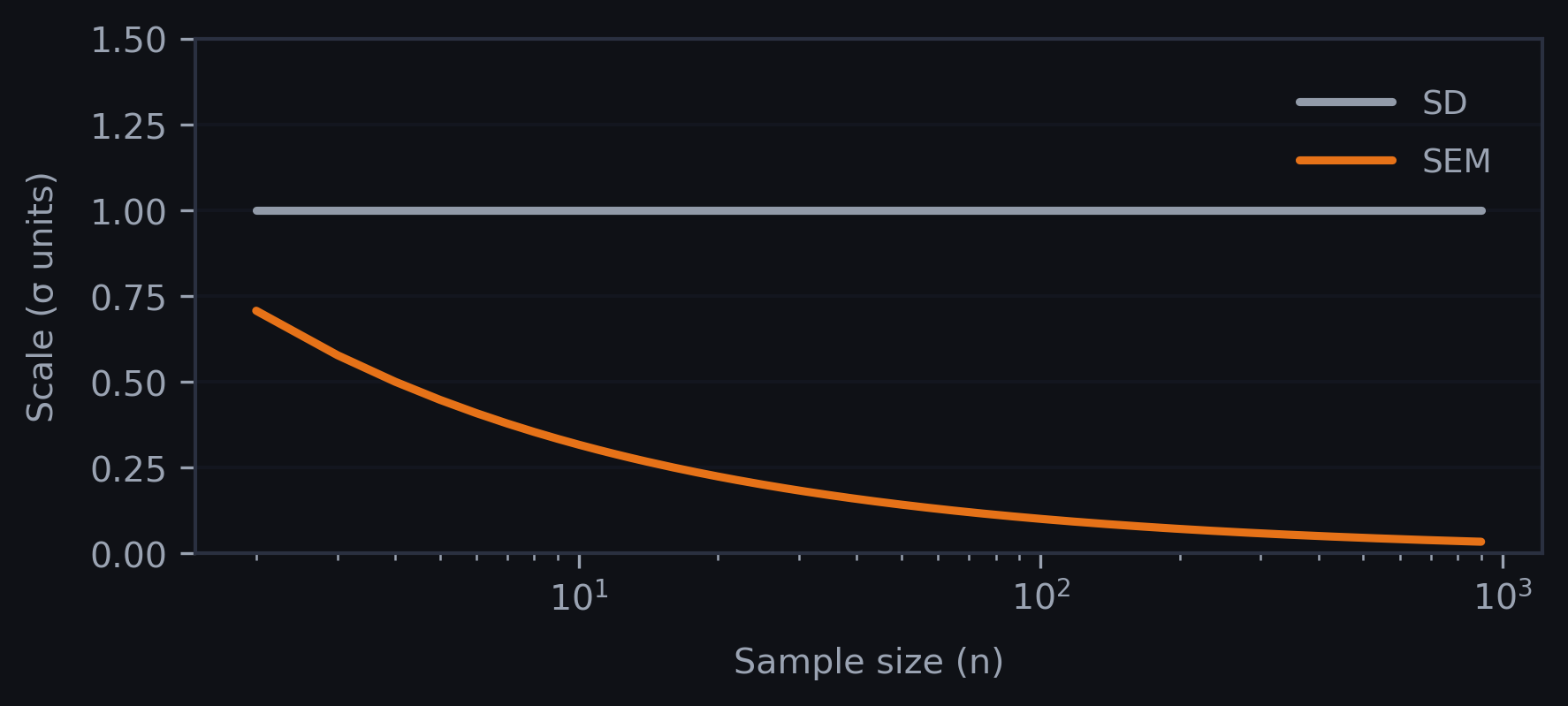
Standard Deviation (SD) and Standard Error of the Mean (SEM) answer two different questions. SD describes the spread of individual data points within a sample. It quantifies variability among subjects or measurements and does not systematically shrink as sample size increases. SEM measures the precision of the sample mean as an estimate of the population mean. What does that mean? It means that if I repeatedly sampled the same population and recalculated the mean each time, SEM tells me how much those sample means would typically vary around the true mean. It is derived from SD by the relation SEM = SD/√n, so it decreases as sample size increases.

This mathematical relationship creates a powerful visual effect: with larger n, and even at one, SEM bars are quite small even when the underlying observations are widely spread out.

Visual deception

To show how this impacts error bars, we can make a few plots with simulated data. Below you can see the difference - each color dot represents a group of measurements (5 groups with 5 measurements each). While the SD preserves the overall variance in data, the SEM shows that all groups converge to a similar average.

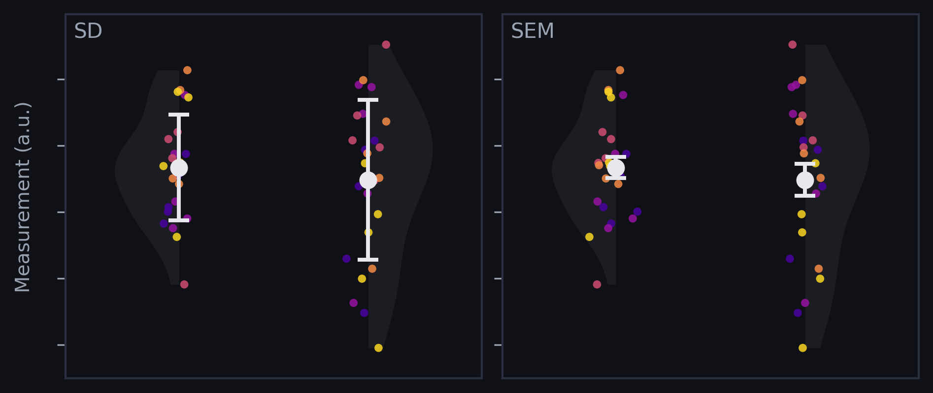
With SD error bars, overlap between groups is often clear. With SEM error bars, overlap can appear reduced simply because the bars are scaled down by √n. This matters because many readers use error bars as a quick proxy for if an effect is real, even though researchers routinely misinterpret what different error bars imply (Belia et al., 2005).

Unintentional misuse under publication pressure

Outside of people misinterpreting error bars, the publishing researchers can also mess it up. Misuse of SEM as a descriptive statistic is often framed as a technical error and it shows up across fields.

In four anaesthesia journals (2001), 23% of articles inappropriately used SEM to describe sample variability (198/860) (Nagele, 2003).
In three selected cardiovascular journals (2012), 64% of assessed articles contained at least one instance of incorrect SEM use for description, with especially high rates in basic science papers compared to clinical papers (a whopping 7.4 times higher) (Wullschleger et al., 2014).
In four obstetrics and gynecology journals (2011), the overall misuse rate reported was 13.6% (Ko et al., 2014).

Guidelines have existed for years, yet somehow this still goes wrong. Even I probably have been at fault of making a mistake, and I think it can come down to a combination of misunderstanding the statistics at play, and seeing that the SEM looks better and always preferring it for this reason.

Toward honest visual communication

If we want to solve this, we need to first make sure we're picking the right error bars for the right question. The next, even more important part, is to label them properly in the caption or figure somewhere. My takeaways are:

Researchers: Use SD (or IQR) to describe variability in the observed sample; use confidence intervals when you want to communicate uncertainty about an estimated parameter
Editors and reviewers: Require figure legends to state what error bars represent, and push authors toward plots that show the data more directly when feasible (Weissgerber et al., 2015). (I had to report what my error bars were in nearly every paper I published!)
Readers: Treat small error bars as SEM unless the caption clearly says otherwise, or you can see the variation in the data somewhere to confirm.

SD is tied to the spread of individual outcomes. SEM is tied to the spread of the mean across (hypothetical) repeats of the study (Curran-Everett & Benos, 2007). Both can be useful, but they communicate different things. In many real-world contexts, individual variation can be the point: patients, cells, and organisms experience outcomes one-by-one, not as an abstract mean.